
By: A.R.M. van der Last and G. Lettings.
Reprinted from: Water Science & Technology: Water Science & Technology.
Abstract
This paper describes experiments with domestic sewage using a 120 litre expanded granular sludge bed (EGSB) reactor and a 205 litre fluidised bed (FB) reactor. Presettled domestic sewage was used in the experiments, because these reactor systems are inadequate in removing SS. Compared to conventional UASB reactors, the advantage of EGSB systems is the significantly better contact between sludge and wastewater.
A bath recirculation system was used to assess the maximum achievable removal of the different COD fractions under EGSB and UASB conditions.
The results obtained with the EGSB reactor reveal a removal efficiency of 90% with respect to the maximum obtainable efficiency of the soluble COD fraction under dry weather conditions. This efficiency can be obtained at hydraulic retention times (HRT) exceeding 3 hours. Even at HRT’s ranging from 2 – 1.5 hours, still 84% – 77% of the maximum possible removal efficiency as assessed in batch recirculation experience can be achieved at temperatures exceeding 13 °C.
The advantage of EGSB systems is the high volumetric loading rate that can be applied while maintaining a high removal of the dissolved COD fraction. Moreover, little if any accumulation of inert suspended solids occurs in the sludge bed.
On the other hand, the poor removal of suspended solids can be considered as a disadvantage of these systems in treating domestic sewage.
Conventional FB systems using sand as carrier material were shown to have little prospect or treating settled domestic sewage, because hardly any methanogenic activity will develop in such a system.
However, it was also found that a very satisfactory quality granular sludge developed on settled sewage when operating FB systems in a mode similar to EGSB systems. This granular sludge appeared to be of a quality equal or even better than that of granular seed sludge, cultivated in a UASB reactor treating papermill wastewater.
Keywords
Anaerobic Treatment; Domestic sewage; Moderate climate; EGSB; FB; Granular bed expansion
Nomenclature
| COD | [mg/1] | Chemical Oxygen Demand |
| CODtot | [mg/1] | COD of the total sample |
| CODf | [mg/1] | COD of a paper filtered sample |
| CODm | [mg/1] | COD of a membrane filtered sample |
| CODss | [mg/1] | COD present as coarse suspended solids |
| CODcol | [mg/1] | COD present as colloidal matter |
| CODsol | [mg/1] | COD present as soluble fraction |
| CODvpa | [mg/1] | COD present as volatile fatty acids |
| d | [m] | diameter reactor part of the column |
| ds | [m] | diameter settling part of the column |
| Es/s | [%] | removal efficiency related to CODsol |
| Et/t | [%] | removal efficiency related to CODtot |
| Ess | [%] | removal efficiency related to CODcol |
Introduction
As a result of the development of new advanced reactor systems with an excellent biomass retention, such as UASB1, FB2, AAFEB3 and AF4 reactors, the anaerobic process now offers great opportunities for the treatment of a large variety of medium and low strength wastewaters. As a consequence of the high biomass concentrations in these reactors (30 g VSS/1), it is possible to maintain a sufficient amount of very slow growing methanogenic bacteria in the reactor. These organisms are necessary for removing the organic pollutants (COD) from the wastewater, as they fulfil the terminal COD removal step in the anaerobic digestion process. Obviously, the big challenge for engineers is to demosntrate the applicability of these anaerobic reactor systems for the treatment of domestic sewage, especially when used under moderate climate conditions.
Since 1976, research has been done at the Agricultural University of Wageningen on the anaerobic treatment of raw domestic sewage using UASB reactors. First, experiments were done with pilot scale reactors (0.12 m3, 6m3), seeded with flocculant sludge, to study its applicability under tropical conditions (T constant at 20 °C). Later, its applicability was investigated at ambient temperatures (in the Netherlands: summertime 15- 20 °C, wintertime 6-9 °C) (Lettings et al., 1981; de Man et al., 1986). The results, obtained with a 0.120 m3 granular bed UASB reactor, demonstrated that a total COD removal efficiency ranging from 45 to 75% can be achieved at 12-18 °C and at 4-8 hours hydraulic retention time (HRT). However to achieve the same effluent values at temperatures below 10 °C, the HRT has to be increased to 9-14 hours. The accumulation of suspended solids becomes significant at lower temperatures due to very slow hydrolysis of the entrapped solids.
Results obtained in upscaled reactors (6 and 20m3), seeded with granular sludge, gave distinctly lower efficiencies, which could be attributed to a poorer sludge water contact and decreased removal of suspended solids (de Man, 1986). De Man performed tracer-pulse experiments in the 20m3 granular bed UASB reactor, equipped with two inlet points (0.67/m2). which -if desired- could be rotated at speeds up to 0.25 rpm. At an HRT of 13-14 h and a rotation speed of 0.1 rpm there was no dead space in the reactor amounted to 17 and 40% respectively of the total reactor volume. It was found that this 20m3 UASB reactor only can be used properly, if the right combination of rotation speed and superficial liquid velocity is applied (de Man et al., 1988; de Man, 1990).
In order to improve the sludge water contact, i.e. a more optimal use of the reactor volume, appropriate adjustments should be made to the UASB concept by applying:
- more feed inlet points per square meter;
- a better feed inlet device;
- higher superficial velocities (Vs).
In this study the third adjustment was realized by using the so called EGSB5 system. In this reactor concept a higher superficial liquid velocity causes the granular sludge bed to expand/fluidise, resulting in a better sludge-wastewater contact and less accumulation of flocculent excess sludge between the granular sludge. To achieve sufficient expansion of the granular sludge. To achieve sufficient expansion of the granular sludge bed, the superficial liquid velocity in the EGSB system should be in the range of 4-8 m/h (de Man et al., 1988). This was accomplished by designing the reactors with a higher height/diameter ratio and by applying effluent recirculation.
Higher Vs values are also applied in FB systems. However, in these systems a mobile heavy carrier material is employed to immobilize the biomass in thin attached biolayers/biofilms. Normally, the carrier bed is completely (100%) fluidised (Hei jnen, 1984). The minimal fluidisation velocity for silversand is 2.5 m/h. To fluidise this bed completely (100%), a superficial velocity of 24 m/h is necessary. The performance of FB reactors with silversand was extensively investigated at the Gist-brocades company in Delft for treating their own yeast wastewater at 37° C. At big pilot plant scale, the system appeared to be suitable for acidification, methanogenesis on preacidified wastewater as well as for nitrification and denitrification (Hei jnen, 1984; Mulder, 1986).
Both EGSB and FB reactor systems are not expected to be able to remove a substantial amount of coarse suspended solids because of the applied high superficial liquid velocity.
Therefore the systems should focus on:
- the removal of the soluble pollutants from the wastewater (CODsol);
- the maintenance of the methanogenic activity of the biomass (granules/biofilms) over a longer period of time.
This article describes the feasibility of EGSB and FB reactors for treating presettled domestic sewage under Dutch conditions.
The following topics will be described:
- the performance of a 120 litre EGSB reactor, seeded with granular sludge from a full scale UASB reactor, treating papermill wastewater;
- the start-up of 205 litre FB systems at HRT’s of 2.6 and 0.67 hrs and the extent of acidification, that can be accomplished after 105 days of operation.
- the performance of a 205 litre EGSB reactor, started up previously as a FB reactor, with granular sludge, cultivated on presettled domestic sewage;
- batch recirculation experiments to assess the influence of Vs on the maximum possible removal efficiencies for the total COD and the different COD fractions, e.g. the coarse suspended solid, the colloidal and the soluble fraction.
Materials and methods
Reactors
The experiments were carried out in the experimental hall of the Department of Environmental Technology in Bennekom, the Netherlands using 120 litre (R1) and 205 litre (R2 and R3) reactors. The main charactristics of the reactors and used seed sludge/carrier material are summarized in Table 1. Both reactors are presented schematically in Figure 1. The process temperature varied with the ambient temperature.
Table 1 Reactor Characteristics and Used Seed Material
| Reactor characteristics: | used seed sludge/carrier material |
Batch recirculation experiments
The batch recirculation experimental set up was composed of a 6 litre stirred buffer tank and a 1 litre column (inner diameter 0.05 m), which was filled with 0.5 litre (ca. 35 g VSS) granular sludge, adapted to domestic sewage. In these experiments 6 litres of wastewater was recirculated continuosly over the granular sludge bed at Vs= 6 and 1 m/h, vlz. representative for EGSB and UASB reactors respectively. The circulating wastewater was sampled frequently and analysed for CODtot, CODss, CODcol and CODvfa. Most experiments were performed for a period of more than 100 hours, which suffices for the establishment of the “equilibrium state”.
Wastewater characteristics
In all experiments presettled domestic sewage of the village of Bennekom was used. The sewage is collected in a combined sewer system and is continuously supplied to the experimental hall with its original characteristics. The characteristics of the presettled sewage are presented in Table 2. The ambient temperature varied from 15-20°C in summer to 6-9°C in winter. CODtot in the composite samples varied as shown in Figure 2.
Table 2 Characteristics Presettled Sewage
in Bennekomfrom 27/10/86 up to 9/11/89

The continuously supplied influent and the effluent samples were sampled proportional in time to get 48 hour composite samples during the week and 72 hour composite samples during the weekends. The samples were stored in the refrigerator at 4 °C, To prepare the total, filtered and membrane filtered samples, Schuell 595½ paper filters (pore size approximately 4.4 um) and S$S ME25 membrane filters (pore size 0.45 um) were used. CODss and CODcol were calculated subtracting CODf from CODtot and CODm from CODf. CODsol is equal to CODm. The biogas production was measured with a wet test gas meter (company Schlumberger Type 1). The VFA analyses and the biogas composition measurements were made by gas chromatography.
Performance of the 120 litre EGSB reactor (R1), seeded with granular sludge
As seed material 54 litres of “BT” sludge was used (standard acetotrophic methanogenic activity 0.17 g CH,-COD/q VSS.D at 30’C). The experiment lasted 1042 days. At day 977 another 27 litres of granular sludge, cultivated on sugar beet wastewater, was added to the system. The recirculation factor was adjusted in such a way that v. was 5-7 m/h. The average Es/s is presented versus the applied HRT in Figure 3. The efficiency data were obtained at temperatures above 13 °C and are subdivides into three categories, viz. the efficiency under Dry Weather Conditions (DWC, where COD>350 mq/l), under Rainy Weather Conditions (RWC, where COD<250 mq/l) and the conditions in-between, Semi-dry Weather Conditions (SWC). The averages, which are obtained in a state of transition, are not used in this figure. At an HRT of 2 hours, 45% of the soluble fraction could be eliminated under DWC. A further increase of the HRT from 2 to 7 hours hardly has an effect on the Es/s. Under RWC, the Es/s is 22% at the most. However, the COD in the effluent, CODtot as well as CODsol are lower under RWC in comparison to DWC. So the Es/s under DWC is of major concern considering the reactor performance and applicability of these systems, when a specific value is set for the effluent COD.
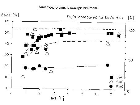
Below 10 °C, during winter time, Es/s drops to 20%. This could be due to the lower methanogenic activity of the granular sludge or a limitation in the maximum possible acidification of the soluble COD fraction in the presettled sewage. More research is needed to explain this problem.
The standard acetotrophic methanoqenic activity of the sludge increased gradually from 0.17 to 0.25 g CH4-COD/g VSS.D at 30°C during the experimental period.
Start-up of two 205 litre FB reactors (R2 and R3) with only presettled sewage as an inoculum
Reactor R2 and R3 were started at HRT’s of respectively 2.6 and 0.67 hours. No seed material was added. Both reactors were filled with 196 kq silversand per m3 reactor. The applied initial superficial liquid velocity was 24 m/h in order to fluidise the silversand bed completely (100%). During the experiment growth or attachment of biomaterial to the carrier material caused a decreasing specific weight of the particles. To retain the particles in the reactor, v. had to be reduced to 12 and 10 m/h respectively. The results obtained with these one step FB systems at a temperature of 10-13 °C (spring time) were quite clear as far as their applicability to pre-settled sewage treatment was concerned. COD reduction they don’t offer any prospect, i.e. Et/t is less than 7% under DWC. The average Es/s also was very low and sometimes even reached negative values.
As a matter of fact, after a biofilm has been developed on the carrier material, the FB’s merely act as a pre-acidification reactor. Under DWC and after 105 days of operation, approximately 59% and 46% acidification relative to the amount obtained in long term batch experiments can be reached in reactor R2 and R3 respectively.
In accordance with the observed very low efficiencies the standard acetotrophic methanogenic activity (at 30 °C) was found to be very low, biogas production in both reactors was nil and the VFA concentration in the effluent increased relative to the influent VFA concentration.
Performance of a 205 litre EGSB reactor (R3) in time
After the start-up experiment of the FB systems, reactor R3 was operated (period b, day 234-511) at HRT’s ranging from 2 to 2.8 hrs (Vs 6-7 m/h ) to act as a preacidification reactor. In the period c (day 522-729) the HRT was gradually increased from 3.3 to 5.8 hrs (Vs 7-8 m/h), which resulted in a start of the biogas production and a sharp increase of the standard acetotrophic methanogenic activity from 0.023 g CH4-COD/g VSS.d at day 497 to 0.16 g CH4-COD/g VSS.d at day 550. The methanogenic activity in this period remained stable at approximately 0.15 gCH4-
COD/gVSS/d. The mean Es/s and Et/t increased as shown in Figure 4. In period d, the HRT was decreased again gradually to 2 h (v. 8-9 m/h) and later on to 1. 5 h (v. 6 m/h) to study the effect of the conditions applied before on the granular sludqe characteristics. Contrary to what was expected, the standard methanogenic activity increased exponentially to relatively very high values, viz. 0.48 q CH4-COD/g VSS.D. After decreasing the HRT to 1.5 h, the standard methanogenic activity stabilised at 0.32 CH4-COD/g VSS.D. The mean removal efficiencies Es/s and Et/t at 2 hours HRT still were respectively 45% and 32% under DWC. At an HRT 1.5 h Es/s decreased to 40%, while Et/t showed the average of 33% under DWC. The development of the standard acetotrophic methanoqenic activity of the granular sludge is shown in Figure 5.
The VSS content of the granular sludge amounted to 70-80%, which is nearly the same as found for granular sludge, cultivated on better degradable wastewaters (Hulshoff Pol, 1986). The fraction of sand in the granules is low. According to our insight the sand acts as growth nuclei in the granulation process.
Batch recirculation experiments
The batch recirculation experiments were carried out to assess the effect of the superficial liquid velocity on the removal of the different COD fractions in presettled domestic sewage. All experiments were performed with 24 hour composite samples. The results of the experiment at v.= 6 m/h and 20 °C are shown in Figure 6. These results can be compared with those found at Vs=1 m/h (see Table 3).
Fig. 5. Standard acetotrophic methanogenic activity at 30 °C of
granular sludge, cultivated in reactor R3 on presettled
domestic sewage in Bennekom
Fig. 6 The course of the different CO values and removal efficiencies as measured in
recirculation batch esperiments
The maximum possible Es/s found for a series of 10 of these trials appeared to be similar for EGSB and UASB systems, i.e.average 54%, standard deviation 12%. As the colloidal fraction is removed partially and the settleability of the SS fraction improves significantly, it is clear that Et/t can be improved distinctly by employing an additional SS-removal step. The maximum achievable total COD reduction of such a combined EGSB-SS-removal system amounts to 78% relative to settled sewage, and 85% relatively to raw sewage, assuming that 33% of the COD can be removed in the presettler.
Table 3 The Influence of v. on the Removal of the Different COD Fractions in
Presettled Domestic Sewage at T =20 °C
| Vs [m/h] |
COD ( t = 0) [mg/l] |
Ess [%] |
Ecol [%] |
Es/s [%] |
Et/t [%] |
| 1 | 421* | 84 | 72 | 44 | 65 |
| 6 | 372° | 0 | 70 | 53 | 42 |
* : d.d. 9/5/88
° : d.d. 17/5/88
Discussion
Table 4 summarizes the results found with one step EGSB systems. The table allows a comparison between the achieved removal efficiencies with the maximum removal efficiencies, as assessed in the batch recirculation experiments (Vs= 6 m/h). A one step EGSB system, seeded with granular sludge, can reach 84% from Es/s, max and 69% from Et/t, max under DWC at T>13 °C. With granular sludge, cultivated on sewage, approximately the same Es/s but even a higher Et/t can be achieved (75%) at 19 °C.
Table 4 The Mean Removal Efficiencies (Es/s), Et/t) as Obtained in
One Step EGSB Systems under DWC
| Reactor Seed* To T HRT VLR (+/-) [*C] [*C] |
Es/s (%) DWC (%max) |
Et/t (%) DWC (%max) |
|||||||
| R1 | BT | 15 | >13 | >3.5 | >2.7 | 51 | (95%) | 34 | (81%) |
| 2.0 | 4.7 | 45 | (84%) | 29 | (68%) | ||||
| 1.5 | 6.3 | 42 | (77%) | 23 | (55%) | ||||
| 1.0 | 9.4 | 33 | (62%) | 16 | (38%) | ||||
| 9 | 2.1 | 4.5 | 20 | (37%) | – | ||||
| 11 | 2.1 | 4.5 | 48 | (89%) | – | ||||
| R3 | -1 | 9.6 | 19 | 2.1 | 4.7 | 45 | (83%) | 32 | (75%) |
| 16 | 1.5 | 5.5 | 40 | (73%) | 33 | (78%) | |||
*: BT : granular sludge grown on papermill wastewater from the full scale UASB installation of Buhrmann Tettenrode in Roermond, the Netherlands.
-1 : self cultivated granular sludge in reactor R3, at the beginning started as a FB reactor, with silversand
as carrier material.
The maximum possible Es/s found for UASB and EGSB systems is similar, but the maximum values for Et/t are significantly higher for UASB systems, viz. 65% compared to 42% for EGSB systems. The reason for this relatively big difference is the poor efficiency for EGSB systems for removing SS.
Nevertheless in view of the higher Vs values applied in one step EGSB systems, these systems offer certain advantages compared to conventional UASB systems:
- little if any accumulation of inert suspended of inert suspended solids occurs in the granular sludge bed. As a result the standard acetotrophic methanogenic activity of the sludge in these reactors increases;
- a better sludge wastewater contact which is especially important for employing the reactor volume as efficiently as possible;
- higher applicable volumetric loading rates (4.7 kg COD/m3.d) as the major concern is the removal of the soluble pollutants;
- a relatively very active granular sludge can be cultivated on settled sewage;
- the settleability of the suspended solid fraction improves.
Incorporation of an EGSB system in an integrated sewage treatment system, can be beneficial, because:
- biodegradable soluble pollutants will be removed without aeratopm (= energy costs);
- the anaerobic EGSB pretreatment step improves the settle-ability of the slowly biodegradable suspended solids and therefore offers the possibility to remove these from the wastewater prior to a post-treatment system for the removal of N (ammonium and nitrate) and P;
- as the suspended solids are not stabilized in the anaerobic EGSB pretreatment step, this offers the possibility to hydrolize acidify the removed suspended solids in a separate sludge acidification system.
The VFA produced can be advantageously used for denitrification and biological P-removal using acinetobacter organisms. Such an approach might become attractive in countries where the removal of total N and phosphate has to be accomplished.
The results obtained with one step FB systems (HRT 2.6 and 0.67 h) at a temperature of 10-13 °C (spring time) clearly show that these systems have no prospect for COD reduction, i.e. Et/t is less than 7% under DWC. The achieved average Es/s also was very low and sometimes even negative. The conclusion is that the FB, started up as described in this study, offers no alternative to the EGSB system.
On the other hand FB systems can be useful for cultivating granular sludge (%VSS > 70%) (HRT 0.67 h) provided the system is operated in the EGSB mode and at an HRT = 3.3-5.8 hrs. The carrier material, e.q. silversand, serves as a growth nucleus. The quality of the cultivated granular sludge appeared to be as good or even better than the granular seed sludge, cultivated in a UASB reactor on papermill wastewater.
Summary and Conclusions
- The maximum possible removal efficiencies for settled sewage in an EGSB system amount to 54% for the soluble COD fraction (Es/s, max) and to 42% for the total COD (Et/t, max), as assessed in recirculation batch experiments.
- The maximum achiebvable total COD reduction of an EGSB reactor system combined with a SS-removal step amounts to 78% relative to settled sewage and 85% relative to raw sewage, assuming that 33% of the COD can be removed in the pressettler.
- Under DWC and when T > 13 °C, one step EGSB systems, seeded with granular sludge, can reach an Es/s of 84% and an Et/t of 69% relative to the maximum possible values, Es/s, max Et/t, max respectively.
- It is possible to cultivate a granular sludge of a relatively high quality (%VSS > 70%) in a FB system (HRT 0.67 h) with silversand, i.e. max. acetotrophic methanogenic activity 0.48 g CH4-COD/g VSS/d) at 30 °C. At HRT= 2h and at T=19 °C, the values for Es/s and Et/t amount to 83 and 76% of Es/s, max and Et/t, max respectively.
- One step FB systems, operated an described in this study, don’t offer any prospect for sewage treatment.
- Littler if any accumulation of inert suspended solids occurs in the granular sludge bed in the EGSB systems, and therefore, the acetotrophic methanogenic activity of the granular sludge in the reactors attains a high value.
Acknowledgements
The active participation in the research of Th. Vens, M. de Wit, R. Sleijster, A. Krom and A. van Amersfoort is gratefully acknowledged.
References
Grin, P.C., Roersma, R.E. and Lettinga, G. (1983). Anaerobic treatment of raw sewage at low temperatures. Proc. European Symposium on Anaerobic Wastewater Treatment (AWWT), Noordwijkerhout, The Netherlands, pp.335-347.
Heijnen, J.J. (1984). Biological Industrial Wastewater Treatment Minimizing Biomass Production and Maximizing Biomass Concentration. Dissertation Technical University Delft, The Netherlands.
Hulshoff Pol, L. (1986). Physical characterisation of anaerobic granular sludge. Proc. Anaerobic Treatment a Grown-Up Technology (AQUATECH 86), Amsterdam, The Netherlands.
Lettinga, G. Roersma, R., Grin, G., Zeeuw, W. de, Hulshoff Pol, L., Velsen, L. van, Hobma, S. and Zeeman, G. (1981). Anaerobic treatment of sewage and low strength wastewaters. Proc, Anaerobic Digestion 1981, Elseiver Biomedical Press, Amsterdam, pp.271-291.
Lettinga. G. & Roersma, R. & Grin, P. (1983). Anaerobic treatment of raw domestic sewage at ambient temperatures using a granular bed UASB – reactor. Biotechnol and Bioengineering. vol. XXV, pp 1801-1723.
Man, A.W.A. de et al (1986). Anaerobic Treatment of Municipal wastewater at low Temperatures. NVZ/EWPCA Water Treatment Conf. Anaerobic Treatment a Grown-up Technology, Amsterdam, pp. 453-466.
Man, A.W.A. de, Last, A.R.M. v.d. and Lettinga, G. (1988). The use of EGSI and UASB anaerobic systems for low strength soluble and complex wastewaters at temperatures ranging from 8 – 30° C. Anaerobic Digestion (Adv. Water Pollut. Control no 5) E. R. Hall & P.N. Hobson 1988, pp. 197-210.
Man, A.W.A. de (1990). Anaerobe zuivering van ruw rioolwater met behulp van korrelslib UASB-reactoren-Werkrapport (in Dutch). Eindrapportage project vakgroep Waterzuivering Landbouwuniversiteit Wageningen.
Mulder, A. (1986). Post treatment of anaerobic sulphide and ammonia containing effluents from methane fermentations in high-rate fluidized bed reactors on laboratory and pilot-scale. NVZ/EWPCA Water Treatment Conf.Anaerobic Treatment a Grown-up Technology, Amsterdam, pp. 413-422.
